
By Andy May
In my last post on Scafetta’s new millennial temperature reconstruction, I included the following phrase which has sparked a lot of controversy and discussion in the comments:
“The model shown uses a computed anthropogenic input based on the CMIP5 models. While they use an assumed climate sensitivity to CO2 (ECS) of ~ 3 ° C, Scafetta uses 1.5 ° C / 2xCO2 to estimate its natural Forces to be considered. “
In the context of the post, I thought the meaning was clear. However, Nick Stokes and others suggested that ECS is an input parameter for the CMIP5 climate models. This is not true, ECS is calculated from the model output. If you pull the above quote from the post and look at it in isolation, it can be interpreted to mean that I changed it to the following, which is clear on this point.
“The model shown uses a calculated anthropogenic input based on the CMIP5 models. However, while using an assumed climate sensitivity to CO2 (ECS calculated from the mean of the CMIP5 ensemble model) of ~ 3 ° C, Scafetta uses 1.5 ° C / 2xCO2 to adjust its estimate of natural forces. “
Then we received criticism of the calculation of the ensemble model mean ECS, some said the IPCC did not calculate an ensemble mean of ECS. This is nonsense, they calculate it in AR5 (IPCC, 2013, p. 818). Part of the table is shown as Figure 1 below.
Figure 1. Part of IPCC AR5 WG1 Table 9.5, page 818. The average ECS of the CMIP5 models is shown below at 3.2 degrees.
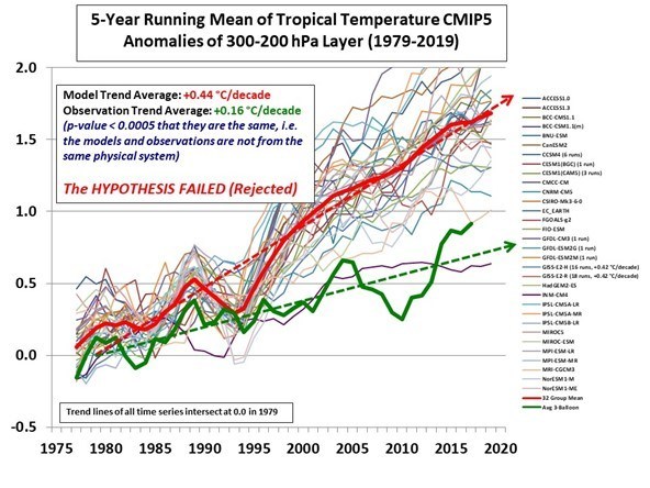
As you can see in Figure 2, most models significantly overestimate warming in the middle to upper tropical troposphere. A pressure of 300 hPa occurs at an altitude of about 30,000 feet or 10 km and 200 hPa at an altitude of about 38,000 feet or 12 km. The top of the troposphere is the tropopause, and in the tropics it is usually between 150 hPa or 14 km and 70 hPa or 18 km.
Figure 2. CMIP5 models compared to weather balloon observations in green in the middle to upper troposphere. The details of why the models statistically fail can be seen in a 2018 article by McKitrick and Christy here.
The purple line in Figure 2 that tracks the weather balloon observations (thick green line) is the Russian INM-CM4 model. As we can see, INM-CM4 is the only model that does pretty well with the weather balloon observations, but it is an outlier among the other CMIP5 models. Since it is an outlier, it is often ignored. In Figure 1 we see that when ECS is calculated from the INM-CM4 output, we get 2.1 ° C / 2xCO2 (degree of warming due to doubling the CO2 concentration). While an ECS of 2.1 since 1979 clearly agrees with the observations, the model average is 3.2. It literally matters that INM-CM4 is one of the few models that passes the statistical test used in McKitrick and Christy, 2018 (see Table 2). That is why I used the word “accepted”. The proof clearly says 2.1, so 3.2 must be assumed. ECS is not an input to the models, but optimizing the models changes the ECS, and the modelers keep a close eye on the value as they optimize their models (Wyser, Noije, Yang, Hardenberg, and Declan O’Donnell, 2020).
McKitrick and Christy have chosen the tropical middle to upper troposphere very carefully and deliberately for their comparison (McKitrick & Christy, 2018). This part of the atmosphere is sometimes referred to as the tropospheric “hot spot” (see Figure 3). Basic physics and the IPCC climate models suggest that this part of the atmosphere should warm faster than the surface when greenhouse gases (GHGs) warm the atmosphere. Dr. William Happer has estimated that the rate of warming of the lower to middle troposphere should be about 1.2 times that of the surface.
Figure 3. The tropospheric “hot spot” from the perspective of the Canadian climate model from 1958 to 2017. By McKitrick and Christy, 2018. Note: mb = hPa. The horizontal scale is the latitude in degrees, the vertical scale is the atmospheric pressure and the Colors are the warming trend rate, the fastest warming is red.
The reason is simple. When the surface is warmed by greenhouse gases, evaporation on the ocean surface increases. Evaporation and convection are the main mechanisms used to cool the surface, as the lower atmosphere is almost opaque to most infrared rays. The evaporated water vapor carries a lot of latent heat with it when it rises in the atmosphere. The water vapor has to rise because it has a lower density than dry air.
As it rises through the lower atmosphere, the air cools down and eventually reaches an altitude where it condenses into liquid water or ice (the local cloud height). This leads to an enormous release of infrared radiation, some of this radiation heats the ambient air and some ends up in space. It is this release of “heat” that is supposed to warm the middle troposphere. Does the “hot spot” exist? The theory says it should if greenhouse gases heat the surface significantly. But the evidence was hard to come by. In Figure 4, the surface temperature from the ERA5 weather reanalysis is plotted against the reanalysis temperature at 300 mb (also 300 hPa or about 10 km). The following curves apply to most of the world. The data comes from the KNMI Climate Explorer. I tend to trust reanalysis data, after all, it is created after the fact and compared to thousands of observations around the world. This diagram is an example, you can easily do others on the website.
Figure 4. ERA5 weather reanalysis temperatures from the surface (2 m) in orange and at 300 mbar (10 km). We expect a faster rate of heating at 300 mbar than at the surface, but instead the rates are almost the same, with the surface rate being slightly higher. The El Niños have a higher rate at 300 mbar, which makes sense.
The warming of the surface ocean should create a “hot spot”. We see this in every El Niño in Figure 4. Surface warming from greenhouse gases should do the same thing, but it is not seen in Figure 4. As mentioned above, the models have been tuned to create an assumed ECS.
discussion
As a former petrophysical computer modeler, I am surprised that CMIP5 and the IPCC average result from different models. It is very strange. By default, the results of several models are examined and compared with observations. This is what John Christy did in Figure 2. Other comparisons are possible but care is taken to highlight the differences. The scattering of the model results is enormous, with some going off the scale in 2010. This is not a data set that should be averaged.
When I was a computer modeler we picked a model that appeared to be the best and average multiple runs of just that model. We never averaged runs from different models, it doesn’t make any sense. They are not compatible. I still think that choosing a model is the “best practice”. I haven’t seen any explanation as to why the CMIP5 produces an “Ensemble Mean”. It seems like an admission that they have no idea what is going on, if they did they would choose the best model. I suspect it’s a political solution to a scientific problem.
The results (see Figures 1 and 2) also suggest that the models are out of phase with one another. Figure 2 shows a stack of spaghetti. Since it is evident that the natural variability is cyclical (see (Wyatt & Curry, 2014), (Scafetta, 2021), (Scafetta, 2013) and Javier’s posts here and here), this strange practice of averaging a phase-shifted model is Die Results completely eliminate natural variability and give the impression that nature does not play a role in the climate. Once you do, you don’t have a valid method of calculating the human impact. You have developed a method that guarantees the calculation of a large ECS. Sad.
IPCC. (2013). In T. Stocker, D. Qin, G.-K. Plattner, M. Tignor, S. Allen, J. Boschung,. . . P. Midgley, Climate Change 2013: The Physico-Scientific Basis. Contribution of Working Group I to the Fifth Assessment Report of the Intergovernmental Panel on Climate Change. Cambridge: Cambridge University Press. Retrieved from https://www.ipcc.ch/pdf/assessment-report/ar5/wg1/WG1AR5_SPM_FINAL.pdf
McKitrick, R. & Christy, J., 2018, A Test of the Tropical Warming Rate of 200 to 300 hPa in Climate Models, Earth and Space Sciences, 5: 9, p. 529-536
Scafetta, N. (2021 Jan 17). Climate dynamics. Retrieved from https://doi.org/10.1007/s00382-021-05626-x
Scafetta, N. 2013, “Discussion about climatic vibrations: General circulation models of the CMIP5 compared to a semi-empirical harmonic model based on astronomical cycles, Earth-Science Reviews, 126 (321-357).
Wyatt, M. & Curry, J. (2014 May). Role for the sea ice of the Eurasian Arctic Shelf in a secularly varying hemispherical climate signal in the 20th century. Climate Dynamics, 42 (9-10), 2763-2782. Retrieved from https://link.springer.com/article/10.1007/s00382-013-1950-2#page-1
K. Wyser, T. v. Noije, S. Yang, J. v. Hardenberg & a. Declan O’Donnell. R. (2020). For increased climate sensitivity in the EC-Earth model from CMIP5 to CMIP6. Geosci. Model Dev., 13, 3465- 3474.
4.8
6
be right
Item rating
Like this:
Loading…
Comments are closed.